Fitting routine for a reliable transient photoluminescence simulation of perovskite films

Introduction

The interpretation of the transient is often not trivial. The simulation of experimental data can make the task easier and allow additionally to gain more insights into relevant processes and parameters.

With this blog post, we present a step-by-step routine developed with the 1-D simulation software Setfos to avoid the introduction of such inaccuracies in the simulation of trPL decays.

Understanding the trPL decay

The amount of radiative and non-radiative recombination can be estimated by the shape of the trPL decay. The radiative recombination rate influences the initial curvature of the decay and depends on the radiative recombination coefficient (B) and the square of the photogenerated carriers. (see Figure 2 left)

The non-radiative recombination rate changes the slope of the trPL curve at longer times (the long-tail), where the dependence on the photogenerated charge carriers is linear (see Figure 2 right). Other parameters affecting the slope are the capture coefficient and the trap density.

Both recombination mechanisms depend on the amount of photogenerated carriers, which varies with the power of the illumination (W/m2). This is determined by the pulse width (the time length with illumination on) and the fluence (nJ/cm2). The former is typically a fixed value of a few nanoseconds, while the latter is varied, to obtain various excitation intensities.

Figure 2. Influence of increasing radiative recombination rate (left) and non-radiative recombination rate on the shape of the trPL decay (right).

Perovskite absorbers are intrinsic semiconducting materials, thus the concentration of both types of charge carriers (holes and electrons) is equivalent to the intrinsic carrier concentration at equilibrium (n0=p0=ni). Whereas under illumination bias the concentration of photogenerated charges will be orders of magnitude larger than the intrinsic carrier concentration (n=p>>ni). In this condition, defined as a high-level injection, it is possible to fit the decay with a bi-exponential equation (see Equation 1), which includes the lifetimes of both the radiative and non-radiative recombination mechanisms.

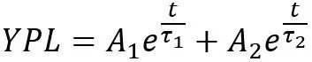
Equation 1. Bi-exponential equation. A1 and A2 are pre-exponential constants, t is the transient time, τ1 and τ2 are the lifetimes of the recombination mechanisms.

Sharp drops in the trPL intensity correlate with shorter lifetimes of the photogenerated charge carriers which depend on processes that limit or delay the emission of photoluminescence from the sample (e.g.: trapping, charge extraction, recombination at the defects, …). These processes are specific to the sample under study, hence, trPL decays are unique for each sample.

It is evident that material properties and methodological parameters have a strong influence on the trPL decay. Establishing a robust routine is essential to set up the simulation reliably.

How to simulate experimental data?

As an example, we consider trPL measurements of a bare perovskite film deposited on glass reported in a recent publication.[Al19] The measurement was carried out with a laser wavelength of 660nm on triple cation perovskite (Cs(MaFa)Pb(IBr), 1.6 eV). The illumination fluence was ranging between 10 and 30 nJ/cm2, while the pulse width is not mentioned. According to the laser datasheet, it is ≤ 2 ns. Only the decay time for the long-tail (corresponding to the non-radiative lifetime) is stated, which amounts to about 1.4 µs. The fitting with the bi-exponential equation confirms the lifetime and it will be used in the rest of the article for comparison purposes. (see Figure 3)

Figure 3. Transient photoluminescence measurement of bare perovskite on glass and its fitting with the bi-exponential equation.

Due to missing details about the experimental illumination conditions and material properties, one is forced to make estimations on the right combination between the two.

Figure 4 shows the bi-exponential fit and simulated trPL decays obtained with increasing illumination fluence. All simulated decays agree with the experimental decay after adapting the electrical properties to the illumination conditions (see Table 1). The long tail of the decay is affected by the non-radiative recombination rate. Because of the linear dependence with the photogenerated charge carriers, the illumination variation has a smaller influence. It follows that the related electrical properties (trap density and capture coefficient) need only minimal change to fit the experimental curve.

On the other hand, the initial curvature of the decay follows the square of the photogenerated charges, which is associated with B. Consequently, B is inversely correlated with the illumination fluence.
This observation highlights the importance to find the right combination between illumination conditions, which is an experimental parameter, and B, which is a property of the material.

Figure 4. Comparison of experimental and simulated trPL decays.

Table 1. Simulation parameters for the trPL decays in Figure 4.

To satisfy this requirement, a fitting routine is suggested (Figure 5) for bare absorbers.
The routine can be described with the following steps:

1.       Set electrical properties of the absorber (such as trap density, capture coefficient, and mobility) except for B. Values should be a rough estimate obtained from scientific literature (they will be revised in the last step);
2.       choose a range of values for B. This material property can vary by order of magnitude. In the case of perovskite, the most conservative range lies within the 1E-10 cm3/s according to the literature;
3.       vary illumination according to experimental conditions. At this point, the goal is to fit the simulation with the initial curvature of the experimental decay. As shown above, B influences the radiative recombination rate, which affects the first nanoseconds of the decay;
4.       fine-tune the electrical properties set at the first step to fit the long-tail of the decay.

Once all the properties are set and the simulated trPL decay fits the experimental decay, the lifetimes should be comparable as well. At this point, the simulation is representative of the experimental conditions. Successive variations to the simulation conditions, either to the excitation conditions or to the material properties, will reproduce a comparable variation in the experimental setup or in the sample.
It is worth mentioning that the material properties we are considering are typically determined with a large tolerance, thus comparisons cannot be in absolute terms, but relative to a set of samples.

Figure 5. Schematic representation of the fitting routine.

Testing the routine

In line with the routine sketched in Figure 5, the initial electrical properties were chosen according to the literature. (see Table 2)
The radiative recombination coefficient was varied within the 1E-10 cm3/s range, but for the sake of this blog post, only the lowest and highest extremes (1.8E-10 and 9.0E-10 cm3/s) will be discussed.

Table 2. Chosen absorber electrical properties to test the fitting routine. Identical trap density, capture coefficient, and mobility values are combined with two different radiative recombination coefficients.

The illumination pulse width was kept at 2 ns, while the illumination fluence was varied in four incremental values (1, 10, 30, and 50 nJ/cm2).
Figure 6 (left) compares the experimental data with trPL decays obtained with increasing illumination for the lowest B value of 1.8E-10 cm3/s. The simulation does not fit the experimental data for any illumination fluence.
Instead, for the highest B value of 9.04E-10 cm3/s, the simulated decay with illumination fluence of 30 nJ/cm2 - which also belongs to the experimental illumination condition stated - fits the experimental one. A finer value optimization of electrical properties related to the non-radiative recombination will be sufficient to fit the decay in the long tail.

Figure 6. trPL decays with increasing illumination fluence for the lowest B (left) and the highest B (right).

With this example, we have shown that by applying the suggested fitting routine, it is possible to quickly find a combination of simulating conditions and material properties that agree with the experimental conditions, without relying on personal experience or knowledge.

Conclusion

Experimental transient photoluminescence (trPL) decays include essential information about the recombination dynamics of the sample under study. Complementing the experiments with simulations can help you in the analysis of the results.
Setting up a simulation with the right settings is not a trivial task due to the large number of interdependent parameters to choose from.
We propose a fitting routine that helps you to quickly define the correct simulation conditions without requiring extensive user experience.

The routine was developed for bare perovskite with the simulation software Setfos. Future applications of the routine will possibly involve bandgap gradients, the influence of interfaces – which are readily available in Setfos – and the inclusion of photon recycling in the optical model. [Aeb21].

Setfos is part of our product for the simulation and characterization of OLEDs, perovskite LEDs, Organic Solar Cells and Perovskite Solar Cells.

References

[Al19] Al-Ashouri et al., “Conformal monolayer contacts with lossless interfaces for perovskite single junction and monolithic tandem solar cells”, En. & Env. Science., vol. 12, 3356-3369, 2019.

[Aeb21] Aeberhard, U. et al., “Reconciliation of dipole emission with detailed balance rates for the simulation of luminescence and photon recycling in perovskite solar cells”, Optics Express 29, 14773, 2021.

Back to the top